Traditionally, the scheduling method used in a small manufacturing shop (let's call it MMS) has been more of guesswork wherein job orders are issued as they come. The main problem with this scenario is that as more job orders enter the shop floor, the larger the work-in-progress (WIP) inventory gets. As a result, idle times for job orders will severely fluctuate contributing to the variability of delivery times for job orders. The bottom line is that supervisors and sales representatives will not have enough data (and confidence) to come up with an accurate completion time estimate for every job order. Often times, they will resort to padding up the completion dates and/or compromising less critical jobs just to avoid late deliveries.
Job Shop Simulation
To demonstrate the phenomenon of fluctuating idle times contributing to the flow times of job orders, two sessions were held in MMS. In both sessions three scenarios were simulated. These simulations are based on the game developed by Dr. James R. Holt (Professor for the Engineering Management department of Washington State University) which was designed to closely resemble the work flow arrangement of job shops.
The arrangement of this simulation is such that four (4) of the participants will act as machine operators doing specialized jobs--that is Operator A cannot act as substitute for Operator B and so forth. One (1) of the participants acted as the scheduler releasing job orders to the shop floor. The remaining participant acted as the monitor responsible for computing each job order's flow days and plotting the data appropriately in a graph.
Scenario #1
This scenario mimics the traditional method of releasing job orders into the job shop floor as they come. The scheduler was given thirty-six (36) pre-filled job orders and was instructed to shuffle them and pick only from the top of the stack during the simulation. Note that all job orders in the stack were designed to require only four (4) operations and should normally be completed within four simulation days. That is, each job order, if properly serviced, should have a flow time of only four (4) days. After the simulation, the data was plotted and was found to resemble the following:
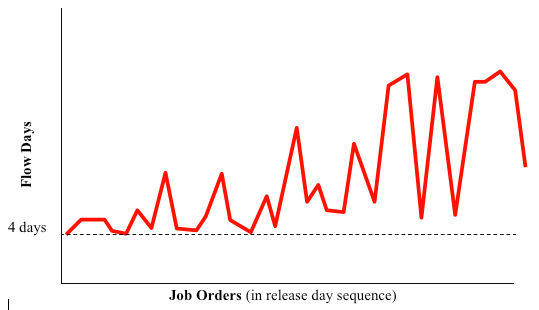
The graph demonstrates that as more job orders are released into the shop floor, the more the workflow is congested contributing to the wild fluctuations of flow times. In the middle of the simulation, participants would have little confidence in answering the question “When will this latest job order be completed?”
After this scenario, the participants were then asked where the problem was. They all noticed that Operator B was the bottleneck. This is actually by design. Operator B represents the most constrained work center in a real-world shop floor environment. In the real world, the cause for this constraint may be anything from limited capability of the work center to high demand for its services. Operator B may be likened to the lathe department of MMS where nearly all of the job orders pass through.
Scenario #2
During the second scenario, the scheduler was given a fresh set of job orders which was exactly the same as the stack given in scenario #1. During this scenario, the participants were asked to work together in arranging the job orders such that they would not cause congestion in Operator B. As with the previous scenario, the scheduler was also instructed to pick from the top of the stack only. After the simulation, the data was plotted and was found to be no different than the graph from scenario 1.
Scenario #3
This scenario now incorporates the Drum-Buffer-Rope (DBR) method into the simulation. The participants were also oriented on the rationale behind DBR as well as given additional instructions to implement it during the game. The scheduler was then given a fresh set of job orders exactly the same as the stacks given in scenarios #1 and #2. The scheduler was then asked to arrange the sequence of cards exactly the same as scenario #1. The reason was to provide a direct comparison of results between DBR, and the method used in scenario #1. After the simulation, the graph plotted resembled the following:
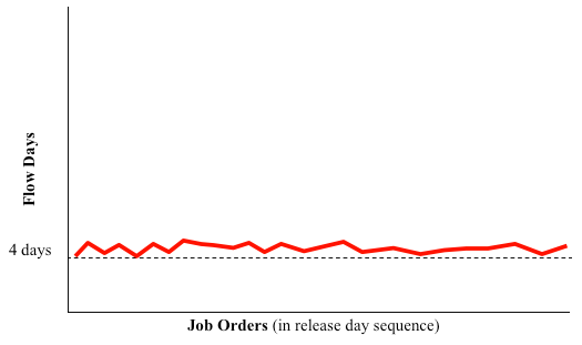
The simulation clearly shows that DBR is a superior method to reduce job order idle time and narrow down the variability of completion times. Utilizing this method, MMS will be able to provide even better delivery-time reliability to its customers.